How To Format Date In Pivot Table

Provisional Formatting in Excel Pivot Table (Tabular array of Contents)

Conditional Formatting in the Pin Table
How to Utilise Conditional Formatting in Excel Pin Table?

Conditional Formatting in the Pin Tabular array

To apply Provisional Formatting in any pivot tabular array, offset, select the pin, then from the Home card tab, select any of the provisional formatting options. If y'all want to format the data with Above Average values under Top/Bottom Rules, choose the option. Afterwards that, from the corner of the prison cell, we will have the Formatting Choice icon; from there, select the formatting dominion for All the cells there in the pivot showing the value as per the defined or selected condition.

How to Apply Provisional Formatting in Excel Pivot Tabular array?

If you want to highlight a detail cell value in the report, use conditional formatting in the excel pivot table. Let's take an example to empathise this procedure.

You can download this Conditional Formatting in Pivot Table Excel Template here – Conditional Formatting in Pivot Table Excel Template

Instance #1

We have given beneath data of a Retail Shop (2 months data).

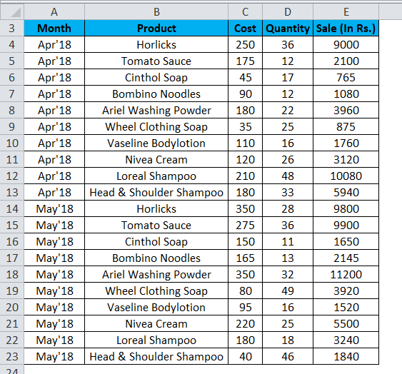
Follow the below steps to create a Pivot Table:

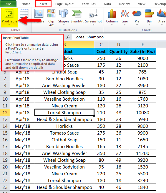
Click on whatever jail cell in the data. Become to the INSERT tab.
Click on the Pivot Table under the Tables section and create a pivot table. Refer to the below screenshot.

A dialog box appears. Click OK.

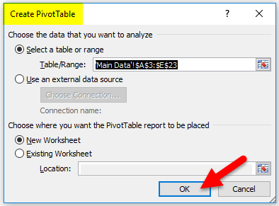
We get the below result.

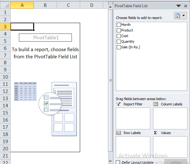
Drag Product field to Rows section, Sales to value section, whereas the Month field to Cavalcade section.

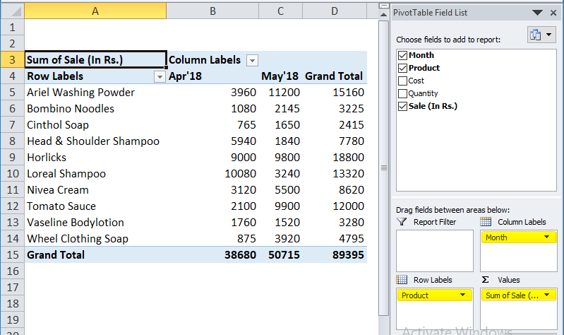
Now we have the Pivot report for month-wise sale. We desire to highlight the products whose auction is less than 1500.

For applying conditional formatting in this pivot table, follow the below steps:

Select the cells range for which you lot want to utilise conditional formatting in excel. We have selected the range B5:C14 here.
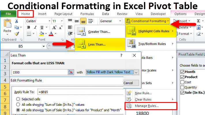
Go to the HOME tab > Click on Provisional Formatting choice under Styles > Click on Highlight Cells Rules option > Click on Less Than option.

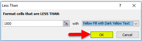
It will open a Less Than dialog box.
Enter 1500 under the Format Cells field and choose a colour as "Yellow Fill with Night Yellow Text". Refer to the below screenshot.

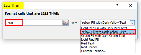
And then click on OK.

The Pivot Written report will wait like this.

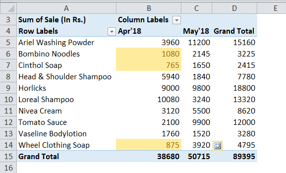
This will highlight all the Cell values which are less than Rs 1500.

But there is a loophole with the condition formatting here. Whenever we make whatever changes in the Excel Pivot information, and then conditional formatting volition not be applied to the correct cells, and information technology might not include the whole new information.

The reason being is when nosotros select a item cell range for applying provisional formatting in excel. Hither we take selected the fixed cell range B5:C14; hence, it would not be applied to the new range when we update the Pivot table.

A solution to overcome the trouble:

For overcoming this problem, follow the below steps subsequently applying conditional formatting in the Excel pivot table:

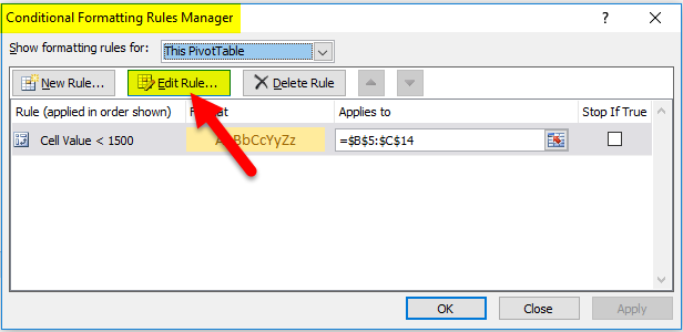
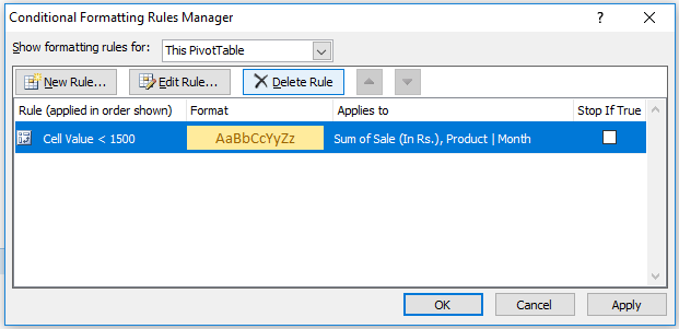
Click on whatsoever cell in the pin table > Go to the Habitation tab > Click on Conditional Formatting choice under Styles option > Click on Manage Rules option.

It will open up a Rules Manager dialog box. Click on the Edit Dominion tab, every bit shown in the below screenshot.

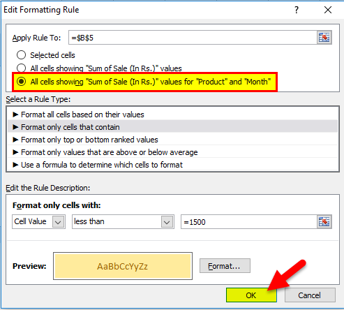
It will open the Editing Dominion formatting window. Refer to the below screenshot.

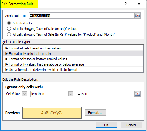
As we tin see in the to a higher place screenshot, Nether Apply Rule To section, at that place are 3 options available:

Selected Cells:This option is non applicable when y'all make any changes in the Pivot data, like add or delete the information.
All cells showing "Sum of Sale" values:This pick might include extra fields similar Grand Totals etc. ,fields which we might not desire to include in our reports.
All cells showing "Sum of Sale" values for "Product" and "Month":This pick restricts with the information and does formatting with cells where our required cells appear. Information technology excludes the actress cells like 1000 Totals etc. This selection is the all-time option for formatting.

Click on the 3^rd selectionAll Cells showing "Sum of Sale" values for "production" and "Calendar month" as shown in the below screenshot ,and and then click on OK.

The below screen will announced.

Click on Apply and and so click OK.

It will utilize the formatting in all the cells with the updated record in the dataset.

Things to Retrieve

If you lot want to apply a new status or alter the formatting color, you can modify these options under the Edit Rule Formatting window.
This is the best choice to present the data to the management and target the specific data which you desire to highlight in your reports.